
String Graph of a Genome
Regular readers are familiar with our explanation of de Bruijn graphs through the following steps -
i) We defined de Bruijn graph for a genome,
ii) We explained that, in the error-free world, de Bruijn graph constructed from short reads sampled from a genome looks identical to the de Bruijn graph of a genome. So, the genome assembly algorithm essentially consists of two steps - constructing de Bruijn graph from short reads (easy, but RAM consuming) and finding the genome sequence from the de Bruijn graph of a genome sequence (difficult, especially for repeat regions).
iii) We explained what impact sequencing errors have on the de Bruijn graph.
We will present String Graph assemblers using similar steps. In this post, we will define string graph for a genome. Please study the following figure carefully.
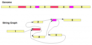
Top part of the above image shows a genome sequence. Yellow regions marked with 1-5 are unique segments, whereas red and purple regions are repetitive segments each appearing twice in the genome. The string graph for the genome is shown in the bottom figure. The graph has seven nodes consisting of five unique regions and two repetitive regions. Multiple appearances of the same repeat all collapse into the same node.
The connectivity between the nodes (edges) follows the same order as the genome sequence. As an example, red repeat region comes after yellow segment 1 in the genome. Therefore, 3’ end of node ‘yellow segment 1’ is connected to 5’ end of red node. It is straightforward to derive the remaining edges based on the genome.
If you remember how de Bruijn graph of a genome looked like, you will notice the following differences.
i) The nodes of de Bruijn graph of a genome consisted of short k-mers of fixed size, whereas nodes of string graph are longer sequences with variable sizes. Therefore, the string graph needs far fewer nodes (and RAM) than de Bruijn graphs.
ii) Typically, the k-mers of de Bruijn graph were shorter than reads. Therefore, de Bruijn graphs were constructed by spitting reads into short subunits. In contrast, nodes of string graph are likely to be longer than NGS read sizes, and thus string graphs are constructed by joining overlapping reads.
Simple, huh? Not so fast. Think about this. When you are are determining overlap between reads to construct the string graph, you have to choose a minimum overlap size as an input parameter. If that minimum overlap size is 1, almost all reads will have some degree of overlap. At the other extreme, the minimum overlap size cannot be longer than the sizes of short reads. So, the overlap size parameter will have some impact on the quality of string graph, just like k-mer size has on de Bruijn graph. It is just that the string graph method shifts the burden on to computation for edges instead of storage for nodes. That is my simple understanding of trade-off between two approaches. (Note - Jared T. Simpson, who developed the SGA algorithm, graciously replied to my question about this issue at a reddit page. Readers are encouraged to take a look.)
One final point - converting a genome into its corresponding string graph does lead to loss of information. If you check the figure presented above, you will find that the string graph is unique for the genome, but given the string graph, many possible genomes (including the original one) can be derived. However, the degree of loss of information is far lower than when a genome is converted into a de Bruijn graph of short k-mer size.