R / Bioconductor (limma)

When I started learning quantum mechanics as a first year Masters student, everything seemed easy. After all, how difficult is it to ‘master’ a few differential equations? My first paper (which happened to get over 400 citations, yay !!) came very quickly, because I did not have enough time to figure out how little I knew. The more I delved into the subject, more I could fathom the depth of my ignorance and appreciate the level of intellect shown by physicists of early 20th century.

The bioconductor package in R gives similar ‘easy’ feeling to new users, because one can go from large amount of experimental data to a table of highly expressed genes by dispensing only a few keystrokes. Nevertheless, keep in mind that those simple R commands hide many complex and conceptually difficult mathematical operations. The next few commentaries on R and Bioconductor will present the general R workflow and, at times, explain what goes on behind the screen.

For a general overview of bioconductor, please review these excellent slides from Ebrahim Emam of EBI. In our forum, we created two threads (limma and oligo) to post other useful online resources as we find them. Those threads will continue to be updated in future.

Let us first study the ‘limma’ package. We like this module the most, because it is useful for both array data and RNAseq data. It identifies ‘fold changes’ from a table of multi-array gene expressions.

A beginner needs to pay attention to three functions in limma -

i) lmFit,

ii) eBayes and

iii) topTable.

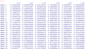
Our input data for today’s analysis consists of a large array with 100 rows (each representing a gene) and six columns (each representing an array measurement). First three columns of the array contain data from one condition (three replicates) and the last three columns contain three replicates of another condition. This website explains how you can create a table with random data for playing with limma.

Here is how part of our input data looks like:

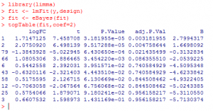
A typical limma session will go like this:

What did we do?

1) We loaded ‘limma’ package.

2) We used ‘lmFit’ function to fit expression to a linear model for each gene and calculate the residual error.

3) Then, we applied ‘eBayes’ function to calculate the likelihood that a residual error would be seen by chance.

4) Finally, we used ‘topTable’ function to produce a table of 10 most differentially expressed genes.

If you try the above example yourself, you will soon find out that we did not give one piece of important information - the ‘design’ array used in lmFit. This array needs to be manually created to describe the design of the experiment. This link explains how the design array is created. We shall add more on this topic in a later commentary.