Using Mate Pair Information in de Bruijn Graphs

This is our last post in the de Bruijn graph series. Although we did not mention explicitly, each of the previous posts was written to present a conceptual building block for the operations of de Bruijn graph-based assemblers. Only thing we did not discuss yet is how the assembly is really done.

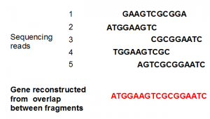
For argument’s sake, imagine you are sequencing a very short gene using the shotgun approach. The sequencer gave you fragments for various parts of the gene, and you have to stitch them together to reconstruct the entire gene.

For a small gene, the stitching together is usually done by aligning all reads and taking the consensus sequence. Sequencing errors are expected to be removed by the consensus generating process.

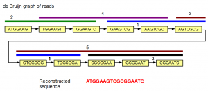
We can also get fancy and do the assembly using de Bruijn graph method. In the following image, the de Bruijn graph for the same five reads is shown. The reads are also displayed above nodes in five identifiable colors.

The de Bruijn graph shown above is linear. Therefore, there is no ambiguity in deciding which k-mer comes after which one. The gene sequence can be reconstructed by starting from one of the graph, and progressively adding extra nucleotides based on subsequent nodes.

The reads in the above example did not have any error. As we explained before, sequencing errors create orphan branches or loops in the de Bruijn graph. Those branches are supported by very small number of reads. So, our quick and dirty de Bruijn assembler needs to include another step (error correction step), where it cleans up all hanging branches or loops supported by handful of reads. The linear chain becomes apparent after the cleaning step, and the gene can be reconstructed.

Conceptually, a de Bruijn assembler for a large genome is not different from the above example. For any genome, we can choose K-mer size large enough (say K=1000 or K=10000) so that the de Bruijn graph turns linear. Once the de Bruijn graph is linear, it is real simple to derive the genome from the de Bruijn graph.

At this point, you are probably going to say - “Hey, wait a sec. How can one construct de Bruijn graph with K=5000, when the reads are not larger than 100 nucleotides.” The answer is simple - mate pairs. You can conceptually think of read pairs that are 5 Kb apart in the genome to produce a giant de Bruijn graph node with size ~5000 nucleotides.

I understand that I am digging a deeper hole for myself. Insert sizes are variable and may not be exactly 5000 nucleotide. Does that mean we are building de Bruijn graph, whose node sizes vary between 4900 nucleotides and 5100 nucleotides?

Instead I like you to forget everything that is said in the last three paragraphs (marked in red). Let me present the matter in traditional way. After you understand what I say below and think deeply about it, you will come to agree with me that large inserts are effectively helping one build de Bruijn graphs with large K-mer sizes, but it is not said that way.

So, how do the de Bruijn assemblers really assemble large genomes from short reads?

Step 1. A giant de Bruijn graph is constructed from all reads, but mate pair information is ignored first. This is because de Bruijn graphs cannot preserve sequence space correlations. So, there is no way to naturally incorporate mate pair data within de Bruijn graph.

Step 2. The de Bruijn graph is cleaned from all possible sequencing errors. That means all hanging branches and loops supported by few reads are purged.

Step 3.Some parts of the giant graph can be linearly traversed. Efforts are made to simplify those linear parts as much as possible. After this step, we may get few contigs longer than 1Kb from non-repetitive regions of the genome. Other parts of de Bruijn graph having junctions (representing repetitive regions) cannot be simplified. Therefore, contig size never gets too large at this stage for complex eukaryotic genomes.

Step 4.Mate pair information is introduced next. An attempt is made to find linear paths through the graph that satisfy restrictions imposed by read pair distance on two ends. A good example of how that is done is provided in the Velvet paper. Please jump to their Breadcrumb: Resolution of repeats with short read pairs section.

The contig/scaffold size after Step 4 depends on repeat structure of the genome and mate pair insert sizes. Some less complex genomes may be derived with insert sizes 5 Kb long. Other complex genomes may require inserts of size 20 Kb. This is where the three red paragraphs become handy. In our original description of de Bruijn graph, we started with building de Bruijn graph for the genome itself. I believe (although I have no calculation to prove this assertion) if the de Bruijn graph of a genome is simple and linear with K-mer size=5000 nt, one should be able to assemble it from insert sizes of 5Kb length. On the other hand, a complex genome with many 5Kb repeat regions will need larger insert sizes (let’s say 20Kb). Please do not use my word on the above matter and DYODD to decide what to do for a sequencing project.