The New K-mer Counter and a Genome Assembly - (ii)

In the last commentary, we have shown a few examples of doing k-mer counting with the new super-efficient program - kmc-2. This commentary will provide the context. Readers unfamiliar with how to interpret k-mer distributions of short reads are also encouraged to go through an old blog post - Maximizing Utility of Available RAMs in K-mer World.

Here is our story. We started assembling two sets of Illumina libraries discussed in previous commentary using Minia and noticed something odd. At first, we assembled the set2 (see previous commentary for reference) at k=63 using Minia. Total size of all assembled contigs came to be around 700Mb with N50=982. So far, so good.

Another bioinformatician helped us assemble set1 and set2 together with Minia. Since the depth of sequencing was very high, we chose to do this assembly at k=73. The total assembly size came to be roughly the same, but, quite puzzlingly, N50 dropped to 219 !

To figure out what was going on, we took set2 and did k-mer counting at k=63. The distribution came out to be usual (unimodal with peak around 23, ignoring the noise peak near count=1). As explained in the earlier commentary, the location of the mode of the distribition is attributable to the depth of sequencing and the amount of repeats in the genome. The peak at 23 was somewhat low given how deeply this genome was sequenced (~50 was expected), but we also knew that this organism had extensive duplication. Therefore, there was nothing odd with the k-mer distribution as such.

-—————————————————-

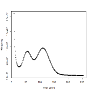
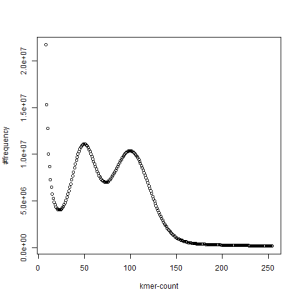
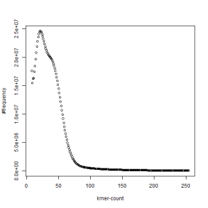
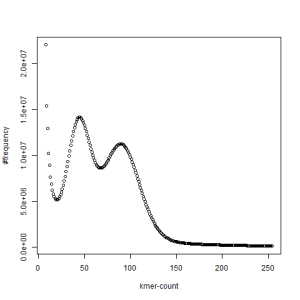
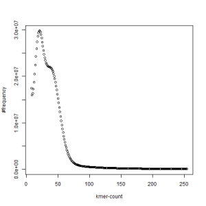
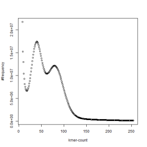
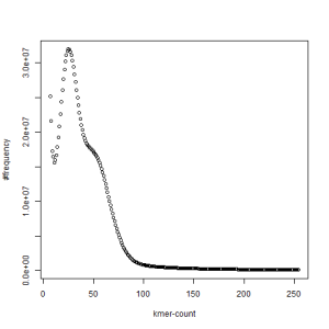
Armed with the new k-mer counter, we started to do forensic analysis on the libraries and here is what we found. The following three figures show k-mer distributions for k=21. Especially pay attention to the third chart below.

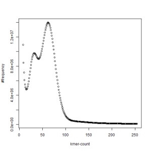
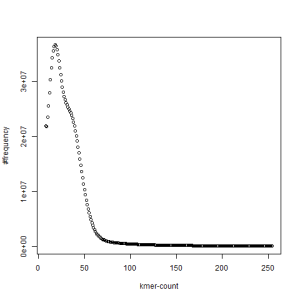
first set, k=21

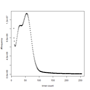
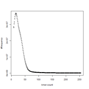
second set, k=21

both sets, k=21

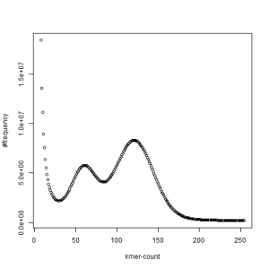
The above chart showing k-mer distribution of the combined libraries has two distinct peaks and one at the right location (~120) derived from the coverage, whereas the other one is at half of that number. The above pattern very likely indicates high degree of heterozygosity in our sample. Two chromosomes in diploid genomes are usually very similar and therefore total k-mer coverage is unimodal. When the difference between the chromosomes start to increase, a second peak appears at location that is half of the primary peak.

We first thought that the two PE libraries (set1 and set2) were prepared with samples from two different animals, but our collaborator confirmed that they were from the same animal. In fact, k-mer distribution from each set also shows two separate peaks, even though those peaks are somewhat less pronounced than when the sets are combined together.

-————————————————————-

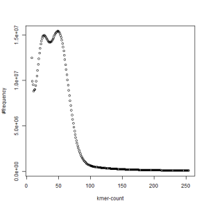
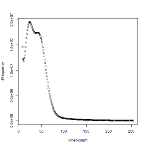
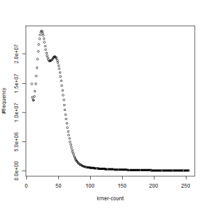
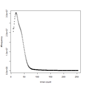
When we plotted the distribution at increasing k-values, quite an interesting picture emerged. First check the following figures and then see the bottom of the post for interpretation.

first set, k=27

second set, k=27

both sets, k=27

-————————————————————-

first set, k=33

second set, k=33

both sets, k=33

-————————————————————-

first set, k=39

second set, k=39

both sets, k=39

-————————————————————-

first set, k=45

second set, k=45

both sets, k=45

-————————————————————-

first set, k=51

second set, k=51

-————————————————————-

both sets, k=63

-————————————————————-

What is going on? We suspect the differences between the two chromosomes are in many short patches and are present all over the genome. Also, we can guess that their relative distances are around 40 (27 + 27/2). So, when we take k-mer distribution at k=21, a large number of k-mers from two chromosomes appear to be identical, thus making the peak at higher coverage taller than the peak at lower coverage. As k is increased from 21 to 27, 33, 39, 45, 51 and finally 63, two chromosomes start to differ everywhere, thus leaving with very few identical k-mers from both copies of the chromosomes. Therefore, the peak at higher value disappears at k=63.

That would certainly be very odd and these charts will keep us awake all night.

Other interpretations are welcome ! Also please let me know, if the descriptions provided above of what we are doing are not sufficient.