R is a very powerful software tool for analysis of biological data. It is an excellent choice for biologists reaching the limits of Excel, because learning R is quite easy. The learning curve is minimal for Matlab or Mathematica users, and R comes with an added benefit of costing less than a cup of coffee. In fact, it costs less than the paper napkin to wipe coffee table - R is free. Primarily for this reason, many users have contributed powerful libraries to R. Those libraries can make statistical analysis of bioinformatic data straightforward. We are particularly attracted to Bioconductor suite of packages.

Where does R fit into the big picture of bioinformatics? In our article titled A beginner’s guide to Bioinformatics part I, we divided bioinformatics skills into five layers. Using R falls into layer 3, which means you mastered layer 1 and are very comfortable with using the web (NCBI BLAST, EBI tools, etc.) for analysis of genomic data. Also, you are able to install and run programs like BLAST, Clustal, Bowtie or Trinity in your local machine (layer 2). Using R needs a bit more skills than installing and running packaged programs, because R also has its own programming language. However, do not let that demoralize you. R language is far easier than PERL or python. R is the easiest of all layer 3 applications, and it will allow you to do many powerful tasks at the cost of little learning.

The purpose of this article is not to have ‘yet another’ introductory tutorial for R, but to guide you through existing online resources to get started. The web is full of excellent introductory articles created by others, and I will refer to the easiest ones that I like the most. I also linked other tutorials and important R sites on the right sidebar, and will continue to add suitable links in the future.

Please follow these steps to use R -

Step 1. Install R

Installing R in Windows or Mac takes only few minutes. If you have not visited the website for R project, please do so now. It has a link for downloading R that takes you to mirror sites from all around the world. I chose the link from Xiamen University, China, because I never heard about the university (pleas pardon my ignorance). After downloading R from the link, I double-clicked on it and the installation took place without any problem.

Step 2. Starting R

After installing R, you will get a small shortcut button on your desktop that looks like this -

Open R by double-clicking the above shortcut and the following R window will appear -

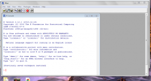
The white screen is the command window for R. You need to type commands in the command window, and R will execute those commands and display results in text or graphical format. For example, if you type command for plotting two sets of data, R will display a beautiful plot.

Step 3. Tutorials for R language

Learning which commands to type is the main challenge, but thankfully excellent tutorials exist online. I found this tutorial to be the best one for someone unfamiliar with R. Following 12 sets of instructions should not take more than an hour.

After finishing the above instructions, please try tutorials at Quick R project. The website is created to help people learn R quickly.

Many other introductory tutorials for R are linked on the right sidebar, but if you finished the above two, I would suggest you to jump straight to Bioconductor. We will discuss Bioconductor packages for Transcriptome analysis tomorrow.

Let me finish this article by giving two examples of using R. The first example is very easy and is p resented to make you feel comfortable with R. In fact, if you finished the above tutorials, you will laugh at me for using the example. The second example is does more complex task by using a library from Bioconductor. You will have to wait till tomorrow to laugh at me for the second example.

Example 1. Simple Calculations

#R can be used as a calculator. if you type any simple

#calculation, R returns the result. No programming needed.

2+3+sqrt(4)

[1] 7

Here we create two vectors x and y, and plot them.

This vector format will be used in R everywhere.

x <-c(1,2,3)

y <-c(10,9,8)

After this command, a new window opens plotting x and y using a line.

plot(x,y,”l”)

Example 2. Processing fastq files

library(ShortRead)

seq <- readFastq(“a.fq”)

primer <- “GGA”

trimmed <- trimLRPatterns(Lpattern=Primer,subject=sread(seq),Lfixed=”subject”)

primer

In the above program, first line opens a library called ‘ShortRead’. If the library is not already installed in your machine, R will find it online and install for you.

The second line loads a fastq file called ‘a.fq’ into an array named ‘seq’. Fastq is a fasta like format typically used for short reads.

The third line creates a string called ‘primer’. It contains the sequence ‘GGA’.

The fourth line goes through all short reads read from a.fq and trims them, if they have GGA or part of it on the 5’ end.

All the above steps are automatically done by R without requiring you to write any complicated python script. Isn’t that cool?

Two questions -

1. In which directory do I save the file ‘a.fq’ for R to open?

Ans. Type ‘getwd()’ in R command window and it will tell you where it picks file from.

How do I get out of R?

Ans. Type ‘q()’ in the command window. You can also use ‘Exit’ from the graphical menu of R to quit.