Errors - Reason for High Memory Usage of de Bruijn Graph-based Assemblers

Bioinformaticians trying to assemble genomes or transcriptomes from large NGS libraries often reach RAM limits of their computers. In this subsection, we examine why de Bruijn graph-based assemblers take so much RAM and what preprocessing of sequencing reads can be applied to get most optimal solution without loss of information.

Let us say you intend to do a genome assembly from 200 million reads in a computer with 128 GB RAM. The amount of RAM is insufficient for your computer, and therefore you need to cut down on the input library size. Intuitively everyone understands that keeping the best reads and removing the worst ones would produce the best result. It is just that the reads do not come marked with good or bad except for the quality score from the sequencers, but the quality scores may not be helpful in improving memory performance. Let us handle the problem in a different way. We shall plot the distribution of k-mers in the data, and show that the distribution has two parts – signal and noise. The goal of best cleaning strategy is to reduce noise and keep signal. We check k-mer distribution, because de Bruijn assemblers view the sequence data in terms of k-mers.

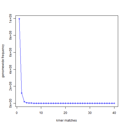
If you remember our earlier discussion on de Bruijn graphs, we first constructed de Bruijn graph of a genome and then showed that de Bruijn graph constructed from short reads is nearly identical to the de Bruijn graph of the underlying genome. In this discussion, we will follow similar approach, but instead of going all the way to de Bruijn graphs, we shall restrict ourselves to the k-mers only. In the above chart, we present the 21-mer distribution of sea urchin (Strongylocentrotus purpuratus) genome. The genome is approximately 900 Mbase long. To prepare this chart, we first split both strands of the genome into all possible 21-mers, and then collected the 21-mers into groups. Most 21-mers were unique in the genome, i.e. they were present only once. Those are 21-mers from non-repetitive parts of the genome. To give you an exact number, 994,401,729 21-mers were present only once in the genome. That is the number you see for x=1 in the following graph. 122,161,264 21-mers were present twice (x=2). 20,077,544 21-mers were present thrice (x=3). So, x axis of the following chart shows multiplicity of 21-mers and y axis shows total count for that multiplicity in the sea urchin genome. At the other end of the curve, 10,000 21-mers were present 67 times in the genome. Those were the repeat regions.

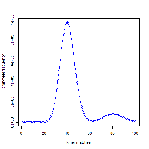
Next we created simulated short reads (100-mer) by sampling the genome uniformly. The reads had 50X coverage of the genome, but all reads were error-free. K-mer distribution of short reads is shown above. We see a large peak at x=40 instead of x=1. What does it mean? By way of construction, every part of the genome is sampled nearly 50 times. A subset of those short reads (about 20%) fell on repetitive regions. Therefore, the unique regions of the genome were sampled 40 times. So, every k-mer that was present once in the genome is now present about 40 times in the simulated short read library. You also see a smaller peak at 80. That comes from those k-mers present twice in the genome. In fact, we checked and found out that the ratio of the peak size at 80 and peak size at 40 in the simulated read data is equal to the ratio of peak size at 2 and peak size at 1 in the K-mer distribution of the genome.

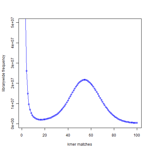
In the next figure, we show the K-mer distribution constructed from short read library of another genome that we are trying to assemble. This is real data from 100 nucleotide Solexa libraries (HiSEQ), not simulated data. You see a peak at around 55 suggesting that the short reads sampled the unique parts of the genome 55 times as expected from simulated data. However, you also see a large peak near 1. That is noise. Please note that Y-axis in the above plot is scaled down.

Why is the noise peak so big? Think about this – every time a read has one nucleotide error, it can result in 21 erroneous 21-mers. Thus, when we look at the k-mer distribution of all reads, errors appear magnified k times. However, there is also memory cost to having those errors, because Each of those erroneous k-mer occupies an unique space in the computer memory. Therefore, much of the RAM is actually wasted by the erroneous k-mers rather than real k-mers. Clearly, a good strategy for cleaning data would be to reduce the noise peak as much as possible. When we trim the edges, it makes sense to check what trimming is doing to the noise peak. If cutting one additional nucleotide does not reduce amount of noise, it is not helping the assembly. I think checking the k-mer distribution is a better measure than using the pre-assigned quality scores from the sequencer.